TA9: Heat Transfer to a Flowing Fluid
1.PROBLEM DESCRIPTION
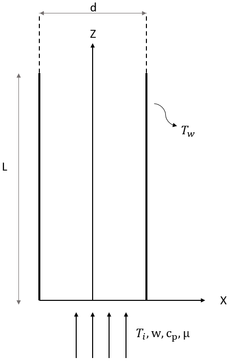
Air in atmospheric pressure is flowin through a tube with diameter of d at a rate of w. The tube has a uniform wall temperature, inlet temperature of the air is given. We are asked to find outlet temperature of the air, inlet and outlet heat transfer rate.
Material Properties |
Geometric Properties |
Loading |
|---|---|---|
c = 100200000 Btu-ft/lbf-hr^2-°F |
L = 5/12 ft |
Tw = 200 °F |
d = 1/12 ft |
Ti = 100 °F |
|
w = \(1.131\times10^{-8}\) lbf-hr/ft |
Before we start, here is the unit conversion for the above table. We will need to use SI units in this problem.
Material Properties |
Geometric Properties |
Loading |
|---|---|---|
cp = 1006.1 J/kg-K |
L = 0.127 m |
Tw = 366.5 K |
d = 0.0254 m |
Ti = 311 K |
|
w = 0.0006 kg/s |
2.MODEL SETUP AND SOLUTION
The following sections describe the setup and solution steps for this tutorial:
2.1. Preparation
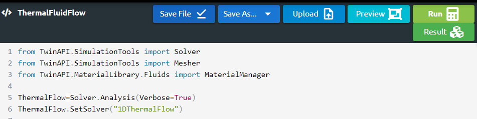
1.First we will import our libraries, that we will use almost in each tutorial, from Simularge Libraries to our empty Python page .
1from TwinAPI.SimulationTools import Solver
2from TwinAPI.SimulationTools import Mesher
Material properties are significant factors that affect the result. Therefore, we should be able to define them easily. TwinAPI’s material library has water, air and oil as fluid. For this problem, we only need air.
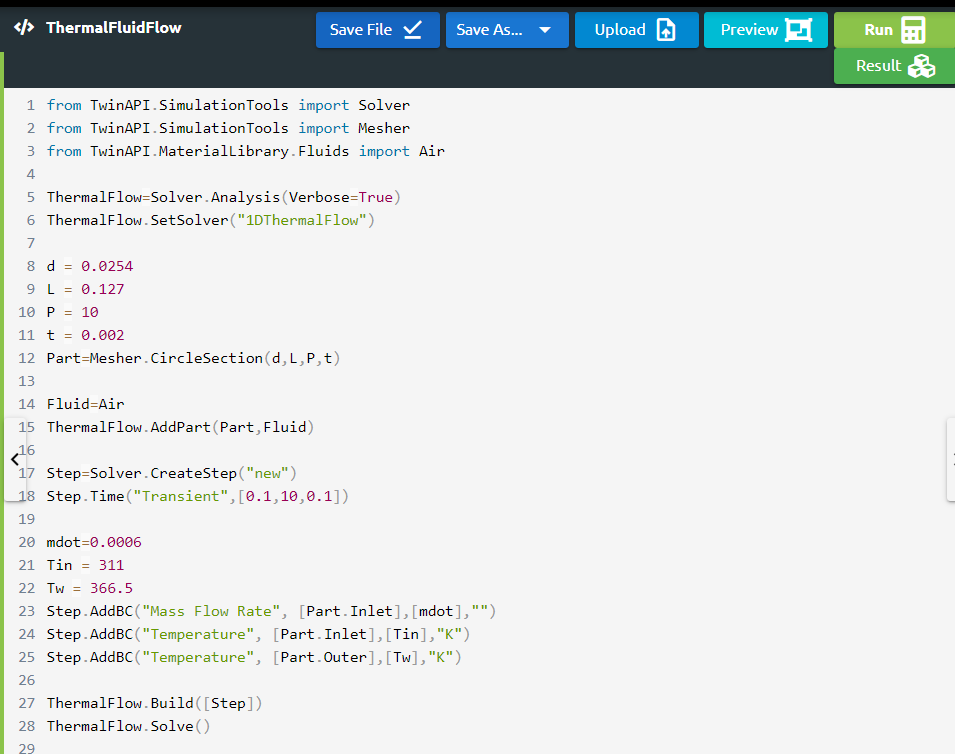
1from TwinAPI.MaterialLibrary.Fluids import Air
2.2. General Settings
After the necessary libraries are imported into the analysis, the analysis is defined.
1.Define the name of the analysis as “ThermalFlow”
1ThermalFlow= Solver.Analysis(Verbose=True)
2.For this problem we will use 1D Thermal Flow as the solver.
1ThermalFlow.SetSolver("1DThermalFlow")
Analysis is defined successfully into TwinAPI system.
2.3. Geometry/Mesh
In 1D Thermal Flow solver, there are three different options for the cross section of the pipe; circular, square and concentric circular section. In this problem we need to a circular section.
1d = 0.0254
2L = 0.127
3P = 10
4t = 0.002
5Part=Mesher.CircleSection(d,L,P,t)
The script given above can be used to create a pipe with circular cross section, which will be used in 1D Thermal Flow solver.
L = length of the pipe
d = diameter of the pipe
P = mesh number
t = thickness of the pipe
We need to define thickness as an input, however it does not affect the result of the problem since the wall temperature of the pipe is uniform.
2.4. Material
Before we start, we need to define the fluid.
1 Fluid = Air
After defining the material into our system, we should combine geometry defined above and material using AddPart.
1ThermalFlow.AddPart(Part,Fluid)
2.5. Boundary Conditions
After adding material and geometry to the analysis, we are ready to set the boundary conditions.
1.First of all, we will create a step with the name “Step”.
1Step=Solver.CreateStep("new")
2.”1D Thermal Flow” is used only for steady state solutions, therefore we do not need to define the type of the solution.
3.Now we define the boundary conditions; mass flow rate, the inlet temperature of the air and the wall temperature of the pipe.
1mdot = 0.0006
2Tin = 311
3Tw = 366.5
4Step.AddBC("Mass Flow Rate", [Part.Inlet],[mdot],"")
5Step.AddBC("Temperature", [Part.Inlet],[Tin],"K")
6Step.AddBC("Temperature", [Part.Outer],[Tw],"K")
2.6. Solution
After defining our boundary conditions, we need to combine our defined domain and the steps containing boundary conditions.To complete this task;
1ThermalFlow.Build([Step])
Now,the problem is ready to be solved.
1ThermalFlow.Solve()
Let’s review what we have done.
2.7. Processing
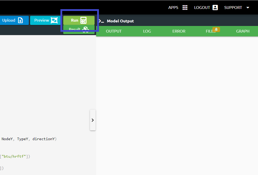
Click Run Button and gears will rotate on the right side while problem is being solved.
2.8. Post-Processing
2.After problem solved;
If we want to see the detailed result of the problem;
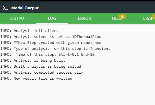
Log tab tells us respectively what happened in the analysis.
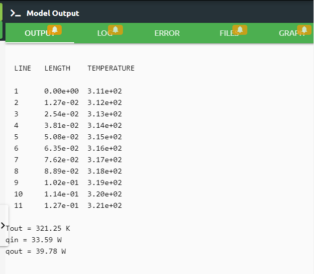
Output tab shows us the results that we desire to see.
 1res=ThermalFlow.Result(Variable="Temperature",Print=True)
 2Tout = res[-1][1]
 3cp = 1006.3
 4
 5Tin_F = (Tin-273.15)*9/5+32
 6Tout_F = (Tout-273.15)*9/5+32
 7Tin_diff = Tin_F*5/9
 8Tout_diff = Tout_F*5/9
 9
10qin = mdot*cp*Tin_diff
11qout = mdot*cp*Tout_diff
12
13print("Tout = {:.2f}".format(Tout), "K")
14print("qin = {:.2f}".format(qin), "W")
15print("qout = {:.2f}".format(qout), "W")
Error tab shows us if there is an error in the script, it tells us what the error is and where it is.
Files tab includes the files imported using Upload button.
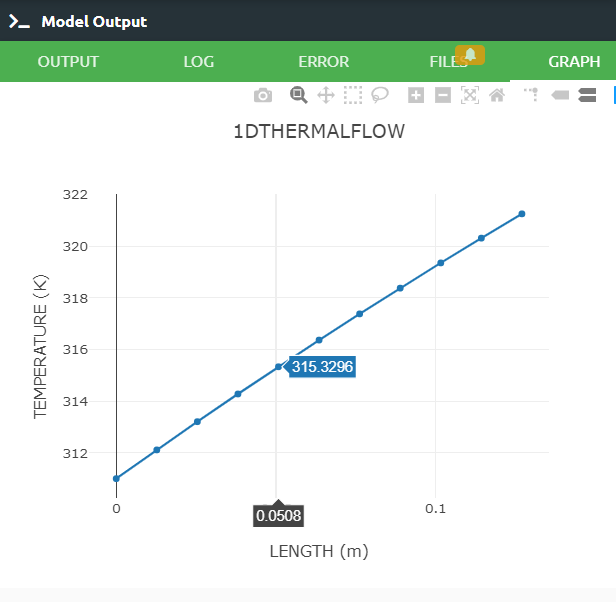
Graph tab shows us analysis result viewed graphically.
 1from TwinAPI.VisualizerTools.Graphics import LineGraph
 2
 3xLocation=res[:,0]
 4xtemp=res[:,1]
 5
 6lineGraph = LineGraph("1DTHERMALFLOW")
 7lineGraph.SetXAxisLabel("LENGTH (m)")
 8lineGraph.SetYAxisLabel("TEMPERATURE (K)")
 9lineGraph.SetXAxisData(xLocation)
10lineGraph.SetYAxisData(xtemp)
11lineGraph.Plot()
3.SUMMARY
In this tutorial, we learned how to set up and solve a pipe flow problem. We also learned how to perform postprocessing in an engineering manner.
The table given below shows comparison of the theoritical result, the result obtained from ANSYS and the result obtained from TwinAPI.
SOLID MODEL |
Target |
ANSYS |
SIMULARGE-TwinAPI |
Ratio: Target/SIMULARGE |
Ratio: ANSYS/SIMULARGE |
|---|---|---|---|---|---|
Tout, K |
123.0 °F = 323.71 K |
122.55 °F = 323.46 K |
321.25 K |
1.01 |
1.01 |
qin, W |
113.28, Btu/hr = 33.2 W |
113.44, Btu/hr = 33.25 W |
33.59 W |
1.01 |
1.01 |
qout, W |
139.33, Btu/hr = 40.83 W |
139.02, Btu/hr = 40.74 W |
39.78 W |
1.01 |
1.02 |
The results given in the table is obtained in TwinAPI with its own correlations. However in the problem description there is coorelation for Nusselt number given for heat transfer coefficient calculations. We used this correlation in the source code of TwinAPI and obtained outlet temperature of the air as 323 K, which is equal to the target outlet temperature.
4. SOURCE CODE
 1 from TwinAPI.SimulationTools import Solver
 2 from TwinAPI.SimulationTools import Mesher
 3 from TwinAPI.MaterialLibrary.Fluids import Air
 4
 5 ThermalFlow=Solver.Analysis(Verbose=True)
 6 ThermalFlow.SetSolver("1DThermalFlow")
 7
 8 d = 0.0254
 9 L = 0.127
10 P = 10
11 t = 0.002
12 Part=Mesher.CircleSection(d,L,P,t)
13
14 Fluid=Air
15 ThermalFlow.AddPart(Part,Fluid)
16
17 Step=Solver.CreateStep("new")
18 Step.Time("Transient",[0.1,10,0.1])
19
20 mdot=0.0006
21 Tin = 311
22 Tw = 366.5
23 Step.AddBC("Mass Flow Rate", [Part.Inlet],[mdot],"")
24 Step.AddBC("Temperature", [Part.Inlet],[Tin],"K")
25 Step.AddBC("Temperature", [Part.Outer],[Tw],"K")
26
27 ThermalFlow.Build([Step])
28 ThermalFlow.Solve()
29
30 res=ThermalFlow.Result(Variable="Temperature",Print=True)
31 Tout = res[-1][1]
32 cp = 1006.3
33
34 Tin_F = (Tin-273.15)*9/5+32
35 Tout_F = (Tout-273.15)*9/5+32
36 Tin_diff = Tin_F*5/9
37 Tout_diff = Tout_F*5/9
38
39 qin = mdot*cp*Tin_diff
40 qout = mdot*cp*Tout_diff
41
42 print("Tout = {:.2f}".format(Tout), "K")
43 print("qin = {:.2f}".format(qin), "W")
44 print("qout = {:.2f}".format(qout), "W")
45
46 from TwinAPI.VisualizerTools.Graphics import LineGraph
47
48 xLocation=res[:,0]
49 xtemp=res[:,1]
50
51 lineGraph = LineGraph("1DTHERMALFLOW")
52 lineGraph.SetXAxisLabel("LENGTH (m)")
53 lineGraph.SetYAxisLabel("TEMPERATURE (K)")
54 lineGraph.SetXAxisData(xLocation)
55 lineGraph.SetYAxisData(xtemp)
56 lineGraph.Plot()
Keywords: 1D Thermal Flow, Pipe Flow, Heat Transfer
Problem Reference: W. M. Rohsenow, H. Y. Choi, Heat, Mass and Momentum Transfer, 2nd Printing, Prentice-Hall, Inc., Englewood Cliffs, NJ, 1963, pg. 168, ex. 7.5
Author: Ilknur Akica