TA12: Thermal Analysis for Shells with Heat Flow and Given Temperature
1. PROBLEM DESCRIPTION
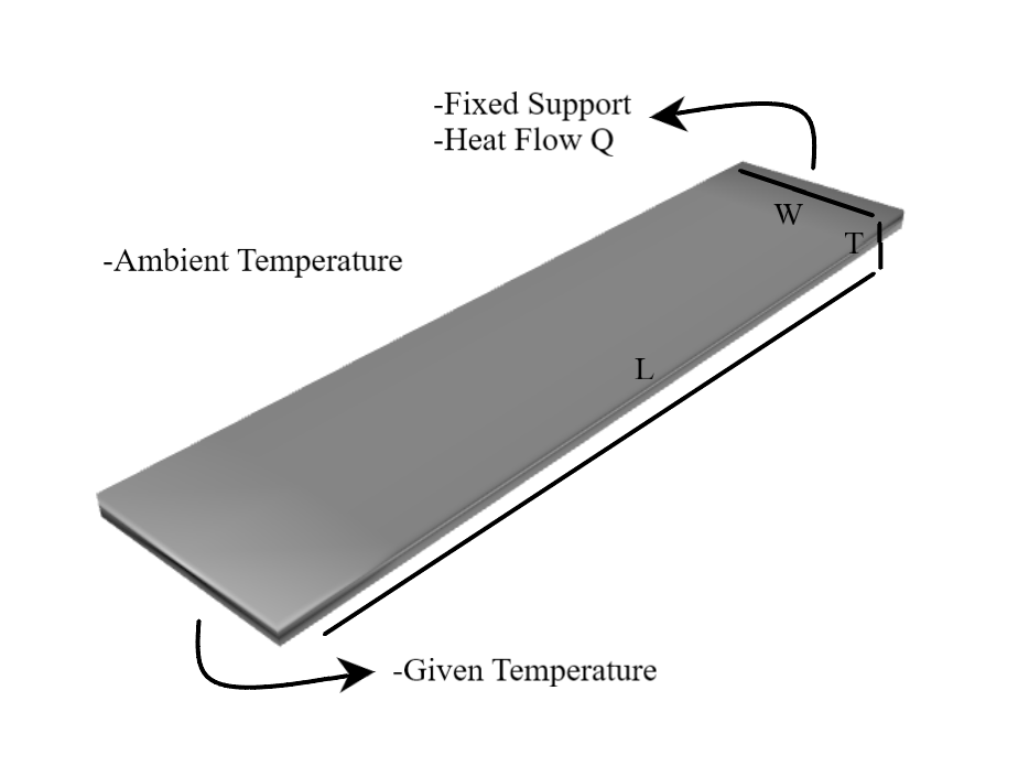
In the problem, an analysis of a plate with a specific temperature on one edge and given heat flow with a fixed support on the opposite edge is analysed. With a given properties and loadings, it is aimed to find the maximum temperature, maximum total heat flux, maximum total deformation, and heat reaction on the plate. Mesh sizes are also specified as 25 mm for the analysis of the problem. The illustration of the problem and given values can be seen in the figure and table below:
Material Properties |
Geometric Properties |
Loading |
|---|---|---|
Thermal conductivity k = 60.5 W/m°C |
Length L = 0.2 m |
Heat flow Q = 5 W |
Thermal expansion α = 1.2e-5 1/°C |
Width W = 0.05 m |
Edge temperature Te = 20°C |
Young’s modulus E = 2e11 Pa |
Thickness T = 0.005 m |
Ambient temperature Ta = 20°C |
Poissons ratio ν = 0 |
1. MODEL SETUP AND SOLUTION
The following sections describe the setup and solution steps for this tutorial:
2.1. Preparation
To run this tutorial;
First of all, TwinAPI is opened and a new project is created as described in the previous tutorials.
Then we import our libraries from the Simularge Libraries. In this project; Solver, Mesher, and Material libraries will be needed. They can be added as before:
1from TwinAPI.SimulationTools import Solver
2from TwinAPI.SimulationTools import Mesher
3from TwinAPI.MaterialLibrary import MaterialManager
4from TwinAPI.MaterialLibrary.Units import units
2.2. General Settings
After the necessary libraries are imported into the code;
The analysis is defined and a name is given. We name our analysis as “ThermalAnalysis”.
Then, solver type is chosen. In this problem, Calculix is preferred for the analysis as a solver.
1ThermalAnalysis = Solver.Analysis(Verbose=True)
2ThermalAnalysis.SetSolver('Calculix')
2.3. Geometry/Mesh
To create a plate, one can use the Mesher Library or upload a .step file of their own CAD geometry. It is more feasible and easier to use box in Mesher Library to draw a plate for this problem.
Because the mesh size is specified in the problem, a function can be written to find the mesh numbers before defining the geometry. The function takes length and node size to return node number for a desired side or length.
1def node_calc(length,node_size):
2    node_number = -(-length//node_size)
3    return int(node_number+1)
Then, the geometry and mesh of the plate can be created by giving the values in the problem.
 1    node_size = 0.025
 2LengthX = 0.05
 3LengthY = 0.005
 4LengthZ = 0.2
 5NodeX = node_calc(LengthX,node_size)
 6NodeY = node_calc(LengthY,node_size)
 7NodeZ = node_calc(LengthZ,node_size)
 8Trans_X = 0
 9Trans_Y = 0
10Trans_Z = 0
11directionX = ''
12directionY = ''
13directionZ = ''
14typeX = 'uniform'
15typeY = 'uniform'
16typeZ = 'uniform'
17plate = Mesher.box(LengthX,NodeX,typeX,directionX,LengthY,NodeY,typeY,directionY,LengthZ,NodeZ,typeZ,directionZ,Trans_X,Trans_Y,Trans_Z)
Note
If there are unclear parts in creating geometry, you can check the Mesher section under the Simulation Tools.
Thus, the plate is created with a name plate using “box mesher” from the given inputs.
Note
The geometry can be also created by importing a CAD file as mentioned. Its code could be written like this after uploading the “plate.step” to the system:
1Plate = Mesher.MeshFromCad('plate.step',10,1,1,SurfaceExtract=True)
The created geometry can be viewed to check before moving to the analysis by clicking the Preview button.

2.4. Material
Material properties are the other type of parameter affecting the results. Using the Material Manager library, a type of the material can be specified.
In this problem, properties are predefined. So, the values in the created material class are written.
1material = MaterialManager.Material("TwinAPI","metal")
2
3material.SetMechanicData("youngsModulus",2e11,units["pa"])
4material.SetMechanicData("poissonsRatio",0)
5material.SetThermalData("expansionCoefficient",1.2e-5,units["1/c"])
6material.SetThermalData("conductivityX",60.5,units["w/mk"])
After defining the material with needed properties for the problem, the geometry and material are combined for the analysis. Then, the analysis is assembled with the defined setup.
1ThermalAnalysis.AddPart(plate,material)
2ThermalAnalysis.Assemble()
2.5. Boundary Conditions
After adding material and geometry to the analysis, we are ready to set the boundary conditions.
First of all, we need to call a method to create a step. Step1’s name can be change.
1Step1=Solver.CreateStep("new")
Then, the time dependence of the problem should be stated. We seek the values at steady-state. Therefore, it is stated as:
1Step1.Time("SteadyState")
Note
If a problem is transient, time dependency of the analysis can be written in a similar manner via the code below. For more detail, you can check the Solver under the Simulation Tools section.
1Step1.Time("Transient",[0,10,0.1])
After that, boundary conditions of the problem should be defined. In our problem, we use ambient temperature and heat flux values as boundary conditions. Also, one edge of the plate is fixed as mentioned in the problem. So, by writing convenient values with proper units, boundary conditions are defined.
1AmbientTemp = 20
2Q = 5
3A = LengthX*LengthY
4q = Q/A
5
6Step1.AddBC("Initial Temperature", [plate.All], [AmbientTemp], "c")
7Step1.AddBC("Temperature",[plate.front],[AmbientTemp],"c")
8Step1.AddBC("Heat Flux", [plate.back], [q], "w/m2")
9Step1.AddBC("Fix",[plate.back],[("Z",0)],"m")
Note
The important point is selecting the appropriate side of the plate geometry while giving the boundary values. For the names of plate (box) surfaces, mesher section can be inspected under the Simulation Tools.
2.6. Solution
After defining our boundary conditions, we need to combine our defined domain and the steps containing boundary conditions. To complete this task;
1ThermalAnalysis.Build([Step1])
Now, the problem is ready to be solved.
1ThermalAnalysis.Solve()
2.7. Processing
Click Run Button and gears will rotate on the right side while problem is being solved. If you have any errors in the code, it will be shown under the Error tab of the Model Output section. By correcting the mistakes, you can get the result.

2.8. Post-Processing
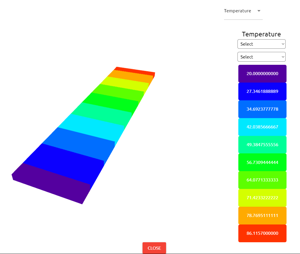
After Problem solved, we can see the results.
Click Result Button
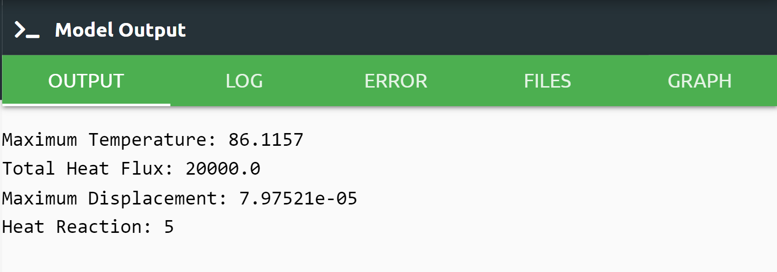
If we want to see detailed result about problem, Output Tab shows us the results that we desire to see.
To see specific outputs of the analysis, we can take desired results at desired locations. By printing selected results, they can be viewed in the output tab.
1Temp=ThermalAnalysis.Result(Variable="Temperature", Loc=[0,0,0])
2Disp=ThermalAnalysis.Result(Variable="Displacement Z", Set=plate.front, Loc=[LengthX,LengthY,LengthZ])
3print("Maximum Temperature:",max(Temp))
4print("Total Heat Flux:",q)
5print("Maximum Displacement:",max(Disp))
6print("Heat Reaction:", Q)
Log tab tells us respectively what happened in analysis.
Error tab shows us if there is an error in script, It tells us what the error is and where it is.
Files tab can upload the files to be imported from the Upload command and check them from Files.
Graph tab shows us graphical analysis results if it is indicated in the code.
3. SUMMARY
In this tutorial, we learned how to set up and solve a problem involving fixed temperature, convection, and fixed edge on TwinAPI. We also learned how to perform postprocessing in an engineering manner.
Table given below shows the comparasion of Ansys Mechanical and TwinAPI results.
Analysed Model |
Target |
ANSYS |
TwinAPI |
ANSYS Error (%): |
TwinAPI Error (%): |
|---|---|---|---|---|---|
Maximum Temperature (°C) |
86.1157 |
86.116 |
86.1157 |
0.00 |
0.00 |
Maximum Total Heat Flux (W/m^2) |
2e4 |
2e4 |
2e4 |
0.00 |
0.00 |
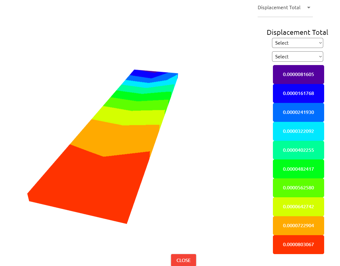
Maximum Total Deformation (m) |
7.93386e-5 |
7.9958e-5 |
7.97521e-5 |
0.78 |
0.52 |
Heat Reaction (W) |
-5 |
-5 |
-5 |
0.00 |
0.00 |
4. SOURCE CODE
 1from TwinAPI.SimulationTools import Solver
 2from TwinAPI.SimulationTools import Mesher
 3from TwinAPI.MaterialLibrary import MaterialManager
 4from TwinAPI.MaterialLibrary.Units import units
 5
 6ThermalAnalysis = Solver.Analysis(Verbose=True)
 7ThermalAnalysis.SetSolver('Calculix')
 8
 9def node_calc(length,node_size):
10node_number = -(-length//node_size)
11return int(node_number+1)
12
13node_size = 0.025
14LengthX = 0.05
15LengthY = 0.005
16LengthZ = 0.2
17NodeX = node_calc(LengthX,node_size)
18NodeY = node_calc(LengthY,node_size)
19NodeZ = node_calc(LengthZ,node_size)
20Trans_X = 0
21Trans_Y = 0
22Trans_Z = 0
23directionX = ''
24directionY = ''
25directionZ = ''
26typeX = 'uniform'
27typeY = 'uniform'
28typeZ = 'uniform'
29plate=Mesher.box(LengthX,NodeX,typeX,directionX,LengthY,NodeY,typeY,directionY,LengthZ,NodeZ,typeZ,directionZ,Trans_X,Trans_Y,Trans_Z)
30
31material = MaterialManager.Material("TwinAPI","metal")
32material.SetMechanicData("youngsModulus",2e11,units["pa"])
33material.SetMechanicData("poissonsRatio",0)
34material.SetThermalData("expansionCoefficient",1.2e-5,units["1/c"])
35material.SetThermalData("conductivityX",60.5,units["w/mk"])
36
37ThermalAnalysis.AddPart(plate,material)
38ThermalAnalysis.Assemble()
39
40Step1=Solver.CreateStep("new")
41Step1.Time("SteadyState")
42
43AmbientTemp = 20
44Q = 5
45A = LengthX*LengthY
46q = Q/A
47
48Step1.AddBC("Initial Temperature", [plate.All], [AmbientTemp], "c")
49Step1.AddBC("Temperature",[plate.front],[AmbientTemp],"c")
50Step1.AddBC("Heat Flux", [plate.back], [q], "w/m2")
51Step1.AddBC("Fix",[plate.back],[("Z",0)],"m")
52
53ThermalAnalysis.Build([Step1])
54ThermalAnalysis.Solve()
55
56Temp=ThermalAnalysis.Result(Variable="Temperature", Loc=[0,0,0])
57Disp=ThermalAnalysis.Result(Variable="Displacement Z", Set=plate.front, Loc=[LengthX,LengthY,LengthZ])
58print("Maximum Temperature:",max(Temp))
59print("Total Heat Flux:",q)
60print("Maximum Displacement:",max(Disp))
61print("Heat Reaction:", Q)
Keywords: Heat Transfer, Conduction, Temperature, Fixed Support, Deformation, Heat Transfer Coefficient
Problem Reference: Any standard Thermal Analysis book
Author: Berkin Aral