TA2: Temperature Distribution Along a Straight Fin

1. PROBLEM DESCRIPTION

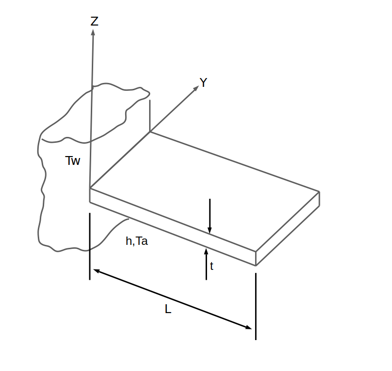
A straight fin with have a rectangular cross-section is fixed from the Wall. Thickness and length of the straight fin are given.The depth of the fin (Y-direction) is arbitrarily selected to be 1 foot.The convection coefficient and ambient temperature of the air around the straight fin are known. The cooling of the straight fin with the convection boundary condition of the air will be examined. We will calculate Heat Flux and temperature distribiton when it comes to steady-state.

Properties and BC Value

Material Properties	Geometric Properties	Loading
k = 15 Btu/hr-ft-°F	L = 4 in = (4/12) ft	Ta = 100°F
h = 15 Btu/hr-ft2-°F	t = 1 in = (1/12) ft	Tw = 1100°F

Figure References: ANSYS Mechanical APDL Verification Manual

2. MODEL SETUP AND SOLUTION

The following sections describe the setup and solution steps for this tutorial:

2.1. Preparation

2.2. General Settings

2.3. Geometry/Mesh

2.4. Material

2.5. Boundary Conditions

2.6. Solution

2.7. Processing

2.8. Post-Processing

2.1. Preparation

To run this tutorial;

1. You must sign up and log in. —->>>>> TwinAPI

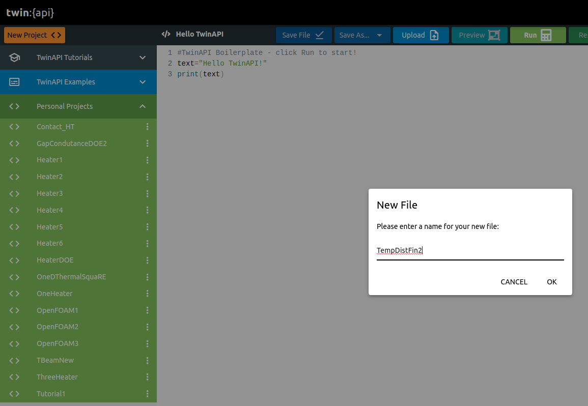
2. After login, Click Personel Projects>>New Project button on the screen and then we will create a project page by giving the project name.

(Let’s name of Analysis “TempDistFin2”)

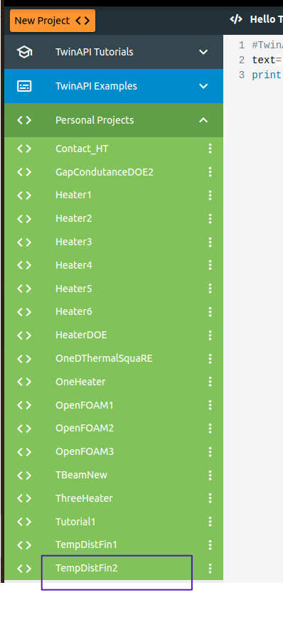
3. You can see the project page on your Personel Project Part.

4. Our Screen is a blank python page without any script. We will be doing a tutorial by using Simularge’s Library.

5. We import our libraries from the Simularge Libraries to our blank Python page that we almost will use in each tutorial.

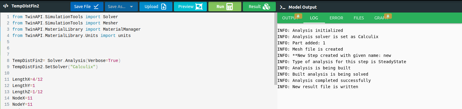
from TwinAPI.SimulationTools import Solver
from TwinAPI.SimulationTools import Mesher

Since we will use air as a fluid in this tutorial, We have to import fluid properties from Simularge’s libraries. (Air is used as a fluid in this problem. We can only choose water apart from air.)

from TwinAPI.MaterialLibrary import MaterialManager
from TwinAPI.MaterialLibrary.Units import units

2.2. General Settings

After the necessary libraries are imported into the analysis, analysis are defined.

1. Defined name of Analysis as “TempDistFin2”

TempDistFin2= Solver.Analysis(Verbose=True)

2. Calculix is used on solid mechanics problems in TwinAPI. Hence, we are defining Calculix to run this analysis.

TempDistFin2.SetSolver("Calculix")

Analysis is defined successfully into TwinAPI System.

2.3. Geometry/Mesh

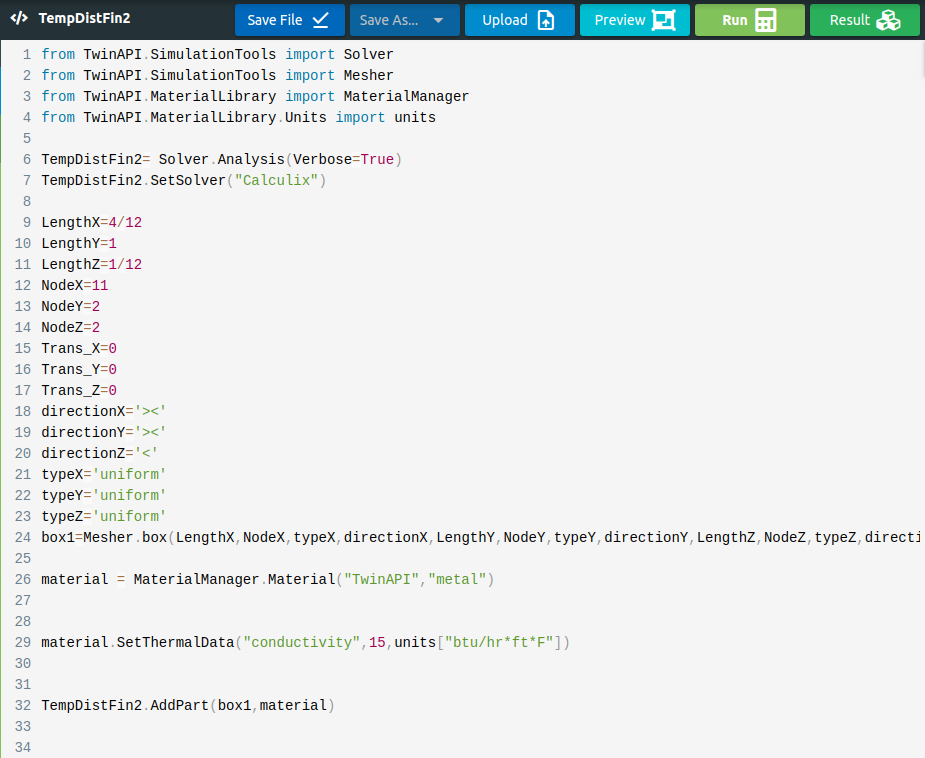
There is two different options to define geometry on TwinAPI System. Create own geometry on TwinAPI by using Mesher Library that belong to Simularge’s libraries or You can import own CAD Geometry.

LengthX=4/12
LengthY=1
LengthZ=1/12
NodeX=11
NodeY=11
NodeZ=2
Trans_X=0
Trans_Y=0
Trans_Z=0
directionX='><'
directionY='><'
directionZ='<'
typeX='uniform'
typeY='uniform'
typeZ='uniform'
box1=Mesher.box(LengthX,NodeX,typeX,directionX,LengthY,NodeY,typeY,directionY,LengthZ,NodeZ,typeZ,directionZ, Trans_X, Trans_Y, Trans_Z)

With the script given above, you can create your box geometry and mesh.

LengthX= Length of X Direction

NodeX= Node Number of X Direction

Trans_X= Translation of X Direction

directionX= Aspect

typeX= Mesh type of X direction.

All of given above is valid for Y and Z Direction.

We create a box geometry that name is “box1” from given inputs.

Note

We told you that you can also create this geometry import 3D CAD file apart from using MESHER. Code should be written like this;

Box1=Mesher.MeshFromCad('Box.step',20000,1,1e4,SurfaceExtract=True)

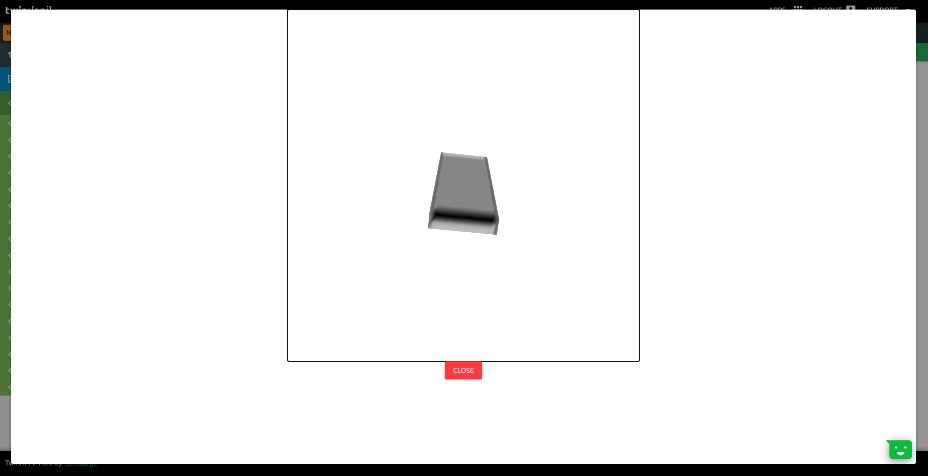
If we are not sure how created geometry and want to see geometry before starting analysis;

Click Preview Button

2.4. Material

Before we started,There are lots of parameters to impact to result of problem. We are going to explain which parameters are requirement for problem first. Later, We would give an parameters instances which can be used.

If your material is isotropic thats means all properties is equal with different direction. However Anisotropic Material Properties is not the same value with different direction. Only Thermal Conductivitiy of material will impact amount of heat transfer in this problem.

We call the Material class in the Material Manager library and name the material “TwinAPI”. At the same time, We give the information that the material behaves as a metal by typing “metal”.

Although not necessary, We have written the conductivity properties in all directions below. But it would be enough if we just write it in the X direction because my material is isotropic..

material = MaterialManager.Material("TwinAPI","metal")


material.SetThermalData("conductivit",15,units["btu/hr*ft*F"])

We will make an example to understand better what can be used parameters in Material Library.

material.SetThermalData("specificHeat",7,units["j/kgk"])

material.SetThermalData("expansionCoefficient",10,units["1/k"])

material.SetGeneralData("density",5,units["kg/m3"])

After defining the material into our system, we should combine geometry define above and material using Addpart method.

TempDistFin2.AddPart(box1,material)

TempDistFin2.Assemble()

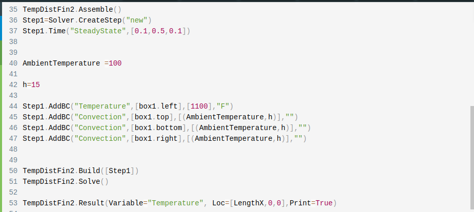
2.5. Boundary Conditions

After adding material and geometry to the analysis, we are ready to set the boundary conditions.

1. First of all, we need to call a method to create a step. Step1’s name can be change.

Step1=Solver.CreateStep("new")

2. We need to choose whether this step is computed depending on time or not.Explained problem is Steady-State. Therefore,below code should be written.

Step1.Time("SteadyState",[0,0.5,1])

If the Problem was Transient,type of problem and time of analysis should be written in a similar manner with below code.

Step1.Time("Transient",[0,10,0.1])

3. The boundary conditions required for the problem are temperature and convection boundary conditions.The ambient temperature and h (Heat Transfer Coefficient) value required for the problem can be defined before the boundary conditions are stated.

AmbientTemperature =100


h=15


Step1.AddBC("Temperature",[box1.left],[1100],"F")
Step1.AddBC("Convection",[box1.top],[(AmbientTemperature,h)],"")
Step1.AddBC("Convection",[box1.bottom],[(AmbientTemperature,h)],"")
Step1.AddBC("Convection",[box1.right],[(AmbientTemperature,h)],"")

2.6. Solution

After defining our boundary conditions, we need to combine our defined domain and the steps containing boundary conditions.To complete this task;

TempDistFin2.Build([Step1])

Now,Problem is ready to be solved.

TempDistFin2.Solve()

Before going to be PostProcess Stage, we can review what we have done.

2.7. Processing

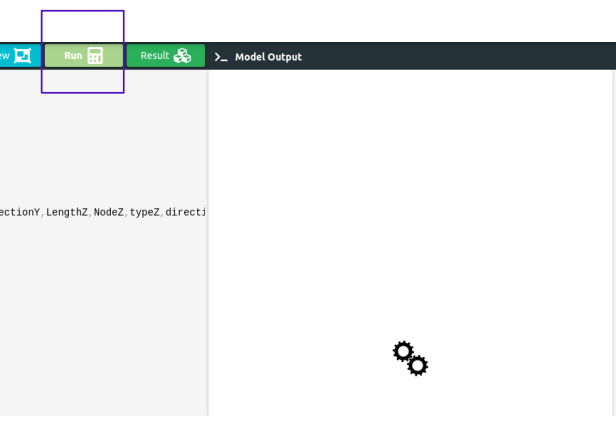
1. Click Run Button and gears rotate on right side while problem is being solved.

2.8. Post-Processing:

.

2. After Problem solved;

We can see result;

Click Result Button

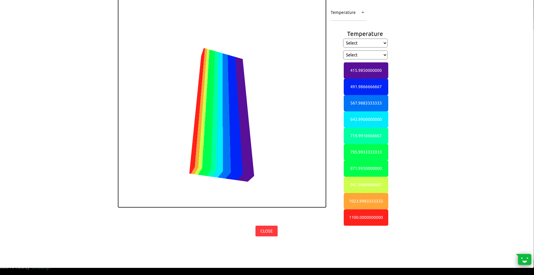
3. If we want to see detailed result about problem;

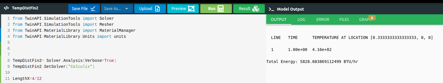
Output Tab shows us the results that we desire to see. If Print=False,We couldn’t see anything in the Output section.

TempDistFin2.Result(Variable="Temperature", Loc=[4/12,0,0],Print=True)

Log tab tells us respectively what happened in analysis.

Error tab shows us if there is an error in script, It tells us what the error is and where it is.

Files tab can upload the files to be imported from the Upload command and check them from Files.

Graph tab shows us analysis result can be viewed graphically. (It will be shown in other examples.)

In the problem example, result information is also given for heat flux. In the post-processing stage, heat flux information cannot be seen at the moment. If you are wondering how we found the Heat Flux given in the Output, it will be enough to write the following after the “TempDistFin2.Solver()” code.

    TempList=[]
    import numpy as np
    for x in np.linspace(0,LengthX,NodeX):

         res=TempDistFin2.Result(Variable="Temperature", Loc=[x,0,0],Print=False)
         temp=res[0,1]
         TempList.append(temp)

    SurfaceList=[]

    for Surface in range(NodeX-1):
        TempList[Surface]
        TempList[Surface+1]
        SurfaceTemp=(TempList[Surface+1]+TempList[Surface])/2

        SurfaceList.append(SurfaceTemp)

    # DeltaX=LengthX/(NodeX-1)
    DeltaX=0.033
    Area=DeltaX+(DeltaX*0.0833)


    EnergyPerSurface=0



    for SurfaceTemp in SurfaceList:
        DeltaT=SurfaceTemp-AmbientTemperature
        HeatFl=h*DeltaT
        EnergyPerElement=HeatFl*Area
        EnergyPerSurface+=EnergyPerElement

    TotalEnergy=EnergyPerSurface*2

    print("Total Energy:",TotalEnergy,"BTU/hr")

3. SUMMARY

In this tutorial, we learned how to set up and solve a problem involving temperature and force convection on a straight Fin in TwinAPI. We also learned how to perform postprocessing in an engineering manner.

With table given below shows that comparasion of Ansys Mechanical Result and TwinAPI result.

Comparison

SOLID MODEL	Target	ANSYS	SIMULARGE-TwinAPI	Ratio: SIMULARGE/Target	Ratio: SIMULARGE/ANSYS
T, °F (at x/length = 0.0)	1100	1100	1100	1.00	1.00
T, °F (at x/length = 0.1)	955	958	957	1.00	1.00
T, °F (at x/length = 0.2)	835	838	837	1.00	1.00
T, °F (at x/length = 0.3)	740	738	737	1.00	1.00
T, °F (at x/length = 0.4)	660	655	654	1.00	1.00
T, °F (at x/length = 0.5)	595	587	586	1.00	1.00
T, °F (at x/length = 0.6)	535	532	531	1.00	1.00
T, °F (at x/length = 0.7)	490	489	488	1.00	1.00
T, °F (at x/length = 0.8)	460	456	454	1.00	1.00
T, °F (at x/length = 0.9)	430	432	431	1.00	1.00
T, °F (at x/length = 1.0)	416	417	416	1.00	1.00
q, Btu/hr	5820	5840	5828	1.00	1.00

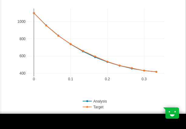
Graph From TwinAPI

4. SOURCE CODE

from TwinAPI.SimulationTools import Solver
from TwinAPI.SimulationTools import Mesher
from TwinAPI.MaterialLibrary import MaterialManager
from TwinAPI.MaterialLibrary.Units import units

TempDistFin2= Solver.Analysis(Verbose=True)
TempDistFin2.SetSolver("Calculix")

LengthX=4/12
LengthY=1
LengthZ=1/12
NodeX=11
NodeY=2
NodeZ=2
Trans_X=0
Trans_Y=0
Trans_Z=0
directionX='><'
directionY='><'
directionZ='<'
typeX='uniform'
typeY='uniform'
typeZ='uniform'
box1=Mesher.box(LengthX,NodeX,typeX,directionX,LengthY,NodeY,typeY,directionY,LengthZ,NodeZ,typeZ,directionZ, Trans_X, Trans_Y, Trans_Z)
material = MaterialManager.Material("TwinAPI","metal")
material.SetThermalData("conductivityX",15,units["btu/hrftf"])

TempDistFin2.AddPart(box1,material)
TempDistFin2.Assemble()
Step1=Solver.CreateStep("new")
Step1.Time("SteadyState",[0,0.5,0.1])
AmbientTemperature =100

h=15
Step1.AddBC("Temperature",[box1.left],[1100],"F")
Step1.AddBC("Convection",[box1.front],[(AmbientTemperature,h)],"")
Step1.AddBC("Convection",[box1.back],[(AmbientTemperature,h)],"")
Step1.AddBC("Convection",[box1.right],[(AmbientTemperature,h)],"")

TempDistFin2.Build([Step1])
TempDistFin2.Solve()

import numpy
xTemp=[]
for xLoc in numpy.linspace(0,LengthX,NodeX):
    xTemp.append(TempDistFin2.Result(Variable="Temperature", Loc=[xLoc,0,0])[0])

Target=[1100.000,955.000,835.000,740.000,660.000,595.000,535.000,490.000,460.000,430.000,416]
from TwinAPI.VisualizerTools.Graphics import LineGraph

fastMultiplePlot = LineGraph("Fast Multiple Plot")
fastMultiplePlot.Plot([{"Analysis": numpy.linspace(0,LengthX,NodeX)}, {"Target": numpy.linspace(0,LengthX,NodeX)}],\
    [{"Analysis": xTemp}, {"Target": Target}])

Keywords: Heat Transfer, Cooling,Convection, Temperature, Heat Transfer Coefficient, Force Convection, Straight Fin, Material

Problem Reference: F. Kreith, Principles of Heat Transfer, 2nd Printing, International Textbook Co., Scranton, PA, 1959, pg. 57, ex. 2-13.