TA13: Thermal Stresses in a Long Cylinder (Under Revision)
1. PROBLEM DESCRIPTION
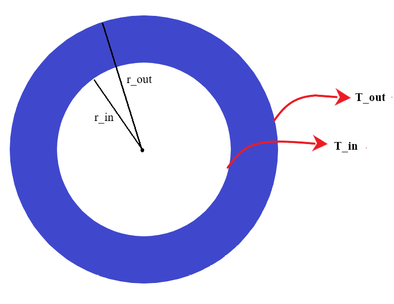
In this problem, inner and outer surface temperatures of a cylinder is given to make thermal and static analysis. With defined properties and specified temperatures, it is aimed to find the temperature distribution through the wall thickness and stresses at the inner and outer surfaces of the cylinder. The illustration of the problem and given values can be seen in the figure and table below:
Material Properties |
Geometric Properties |
Loading |
|---|---|---|
Thermal conductivity k = 8.333e-4 Btu/s-in-°F |
Inner radius r_in = 0.1875 in |
Inner temperature T_in = -1°F |
Thermal expansion α = 1.435e-5 1/°F |
Outer radius r_out = 0.625 in |
Outer temperature T_out = 0°F |
Young’s modulus E = 30e6 psi |
||
Poissons ratio ν = 0.3 |
Note
Axial length is arbitrary and it is chosen as 0.2 inches for the problem.
1. MODEL SETUP AND SOLUTION
The following sections describe the setup and solution steps for this tutorial:
2.1. Preparation
To run this tutorial;
First of all, TwinAPI is opened and a new project is created as described in the previous tutorials.
Then we import our libraries from the Simularge Libraries. In this project; Solver, Mesher, and Material libraries will be needed. They can be added as before:
1from TwinAPI.SimulationTools import Solver
2from TwinAPI.SimulationTools import Mesher
3from TwinAPI.MaterialLibrary import MaterialManager
4from TwinAPI.MaterialLibrary.Units import units
2.2. General Settings
After the necessary libraries are imported into the code;
The analysis is defined and a name is given. We name our analysis as “ThermalStress”.
Then, solver type is chosen. In this problem, Calculix is preferred for the analysis as a solver.
1ThermalStress = Solver.Analysis(Verbose=True)
2ThermalStress.SetSolver('Calculix')
2.3. Geometry/Mesh
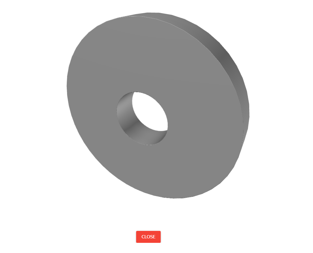
To create a cylinder, one can use the Mesher Library or upload a .step file of their own CAD geometry. It is more feasible and easier to create 2D pipe and then extrude it to make 3D cylinder geometry. For this purpose, we will use Pipe2D and node2Nurbs in Mesher Library to draw a cylinder.
Then, the geometry and mesh of the cylinder can be created by giving the values in the problem.
 1r_i = 0.1875
 2r_o = 0.625
 3n_hoop = 250
 4n_rad = 50
 5typeHoop = "uniform"
 6typeRad = "uniform"
 7dirHoop = ""
 8dirRad = ""
 9angle = 360
10
11pipe=Mesher.Pipe2D(r_i, r_o, n_hoop, typeHoop, dirHoop, angle, n_rad, typeRad, dirRad)
12Path=Mesher.node2Nurbs([[0,0,0],[0,0,0.1],[0,0,0.2]],2,3,4)
13cyl=Mesher.extrusionPath(pipe,Path)
Note
If there are unclear parts in creating geometry, you can check the Mesher section under the Simulation Tools.
Thus, the cylinder is created with a name “cyl” using 2D pipe mesher and extrusion path from the given inputs.
Note
The geometry can be also created by importing a CAD file as mentioned. Its code could be written like this after uploading a “cylinder.step” file to the system:
1Plate = Mesher.MeshFromCad('cylinder.step',20000,1,1,SurfaceExtract=True)
The created geometry can be viewed to check before moving to the analysis by clicking the Preview button.

2.4. Material
Material properties are the other type of parameters affecting results. Using the Material Manager library, a type of the material can be specified.
In this problem, properties of the material are predefined. So, the values in the created material class are written with proper units.
1material = MaterialManager.Material("TwinAPI","metal")
2
3material.SetMechanicData("youngsModulus",3e7,units["psi"])
4material.SetMechanicData("poissonsRatio",0.3)
5material.SetThermalData("conductivity",8.333e-4*3600*12,units["btu/hrftf"])
6material.SetThermalData("expansionCoefficient",1.435e-5,units["1/f"])
After defining the material with needed properties for the problem, the geometry and material are combined for the analysis. Then, the analysis is assembled with the defined setup.
1ThermalStress.AddPart(cyl,material)
2ThermalStress.Assemble()
2.5. Boundary Conditions
After adding material and geometry to the analysis, we are ready to set the boundary conditions.
First of all, we need to call a method to create a step. Step1’s name can be change.
1Step1=Solver.CreateStep("new")
Then, the time dependence of the problem should be stated. We seek the values at steady-state. Therefore, it is stated as:
1Step1.Time("SteadyState")
Note
If a problem is transient, time dependency of the analysis can be written in a similar manner via the code below. For more detail, you can check the Solver under the Simulation Tools section.
1Step1.Time("Transient",[0,10,0.1])
After that, boundary conditions of the problem should be defined. In our problem, we use inner and outer temperatures of the cylinder as boundary conditions. So, by writing convenient values with proper units at inner and outer surfaces, boundary conditions are defined. Also, the cylinder is fixed in the Z direction to restrict its movement in axial direction to see stresses on the geometry.
1T_in = -1
2T_out = 0
3
4Step1.AddBC("Temperature",[cyl.inner],[T_in],"F")
5Step1.AddBC("Temperature",[cyl.outer],[T_out],"F")
6Step1.AddBC("Fix",[cyl.All],[("Z",0)],"")
Note
Selecting the appropriate side of the plate geometry while giving the boundary values is important. For the names of surfaces, mesher section can be inspected under the Simulation Tools.
2.6. Solution
After defining our boundary conditions, we need to combine our defined domain and the steps containing boundary conditions. To complete this task;
1ThermalStress.Build([Step1])
Now, the problem is ready to be solved.
1ThermalStress.Solve()
2.7. Processing
Click Run Button and gears will rotate on the right side while problem is being solved. If you have any errors in the code, it will be shown under the Error tab of the Model Output section. By correcting the mistakes, you can get the result.

2.8. Post-Processing
After Problem solved, we can see the results by clicking the Result button.
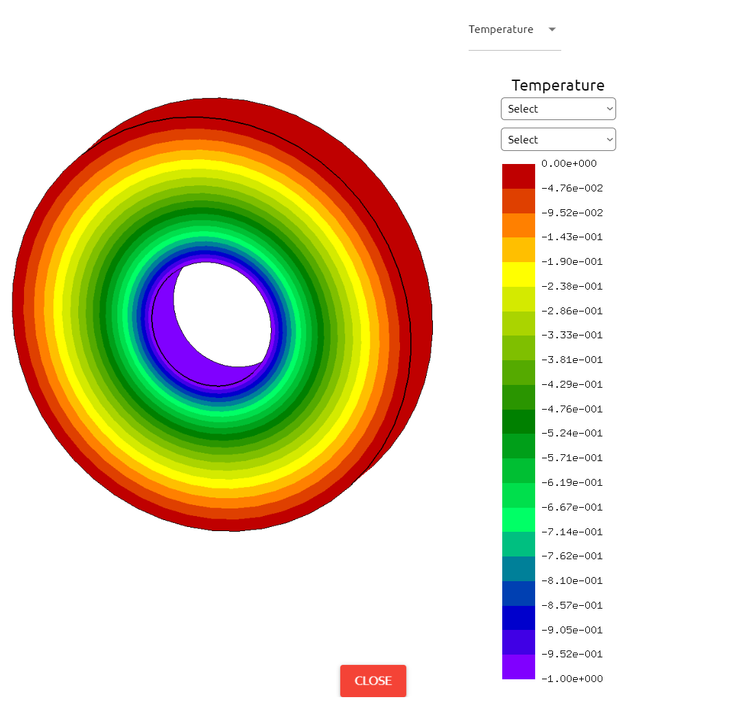
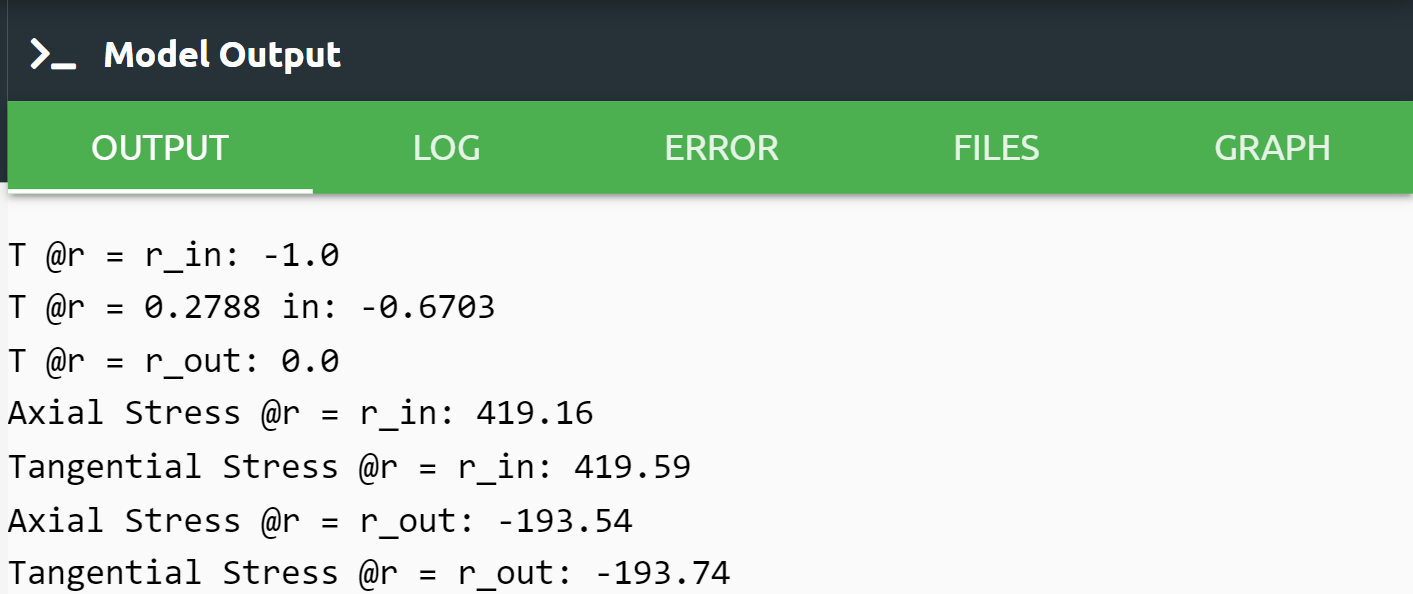
If we want to see detailed results about the problem, Output Tab shows us the results that we desire to see.
To see specific outputs of the analysis, we can take desired results at desired locations. By printing selected results, they can be viewed in the output tab.
 1Temp1=ThermalStress.Result(Variable="Temperature", Loc=[r_i,0,0])
 2Temp2=ThermalStress.Result(Variable="Temperature", Loc=[0.2788,0,0])
 3Temp3=ThermalStress.Result(Variable="Temperature", Loc=[r_o,0,0])
 4StressAxial1=ThermalStress.Result(Variable="Axial Stress", Loc=[r_i,0,0])
 5StressAxial2=ThermalStress.Result(Variable="Axial Stress", Loc=[r_o,0,0])
 6StressHoop1=ThermalStress.Result(Variable="Hoop Stress", Loc=[r_i,0,0])
 7StressHoop2=ThermalStress.Result(Variable="Hoop Stress", Loc=[r_o,0,0])
 8
 9print("T @r = r_in:",max(Temp1))
10print("T @r = 0.2788 in:",max(Temp2))
11print("T @r = r_out:",max(Temp3))
12print("Axial Stress @r = r_in:",max(StressAxial1))
13print("Tangential Stress @r = r_in:",max(StressHoop1))
14print("Axial Stress @r = r_out:",max(StressAxial2))
15print("Tangential Stress @r = r_out:",max(StressHoop2))
Log tab tells us respectively what happened in analysis.
Error tab shows us if there is an error in script, It tells us what the error is and where it is.
Files tab can upload the files to be imported from the Upload command and check them from Files.
Graph tab shows us graphical analysis results if it is indicated in the code.
3. SUMMARY
In this tutorial, we learned how to set up cylindrical geometry and solve a problem involving fixed boundary temperatures to find temperature and stress distributions by using TwinAPI. We also learned how to perform postprocessing in an engineering manner.
Table given below shows the comparasion of Ansys Mechanical and TwinAPI results.
Analysed Model |
Target |
ANSYS |
TwinAPI |
ANSYS Error (%): |
TwinAPI Error (%): |
|---|---|---|---|---|---|
Temperature at r = r_in (°F) |
-1 |
-1 |
-1 |
0.00 |
0.00 |
Temperature at r = 0.2788 in (°F) |
-0.67037 |
-0.67052 |
-0.6703 |
0.022 |
0.010 |
Temperature at r = r_out (°F) |
0 |
0 |
0 |
0.00 |
0.00 |
Axial stress at r = r_in (psi) |
420.42 |
416.06 |
419.16 |
1.037 |
0.3 |
Tangential stress at r = r_in (psi) |
420.42 |
405.31 |
419.59 |
3.594 |
0.197 |
Axial stress at r = r_out (psi) |
-194.58 |
-195.06 |
-193.54 |
0.247 |
0.534 |
Tangential stress at r = r_out (psi) |
-194.58 |
-195.01 |
-193.74 |
0.221 |
0.432 |
4. SOURCE CODE
 1from TwinAPI.SimulationTools import Solver
 2from TwinAPI.SimulationTools import Mesher
 3from TwinAPI.MaterialLibrary import MaterialManager
 4from TwinAPI.MaterialLibrary.Units import units
 5
 6ThermalStress = Solver.Analysis(Verbose=True)
 7ThermalStress.SetSolver('Calculix')
 8
 9r_i = 0.1875
10r_o = 0.625
11n_hoop = 250
12n_rad = 50
13typeHoop = "uniform"
14typeRad = "uniform"
15dirHoop = ""
16dirRad = ""
17angle = 360
18
19pipe=Mesher.Pipe2D(r_i, r_o, n_hoop, typeHoop, dirHoop, angle, n_rad, typeRad, dirRad)
20Path=Mesher.node2Nurbs([[0,0,0],[0,0,0.1],[0,0,0.2]],2,3,4)
21cyl=Mesher.extrusionPath(pipe,Path)
22
23material = MaterialManager.Material("TwinAPI","metal")
24material.SetMechanicData("youngsModulus",3e7,units["psi"])
25material.SetMechanicData("poissonsRatio",0.3)
26material.SetThermalData("conductivity",8.333e-4*3600*12,units["btu/hrftf"])
27material.SetThermalData("expansionCoefficient",1.435e-5,units["1/f"])
28
29ThermalStress.AddPart(cyl,material)
30ThermalStress.Assemble()
31
32Step1=Solver.CreateStep("new")
33Step1.Time("SteadyState")
34
35T_in = -1
36T_out = 0
37
38Step1.AddBC("Temperature",[cyl.inner],[T_in],"F")
39Step1.AddBC("Temperature",[cyl.outer],[T_out],"F")
40Step1.AddBC("Fix",[cyl.All],[("Z",0)],"")
41
42ThermalStress.Build([Step1])
43ThermalStress.Solve()
44
45Temp1=ThermalStress.Result(Variable="Temperature", Loc=[r_i,0,0])
46Temp2=ThermalStress.Result(Variable="Temperature", Loc=[0.2788,0,0])
47Temp3=ThermalStress.Result(Variable="Temperature", Loc=[r_o,0,0])
48StressAxial1=ThermalStress.Result(Variable="Axial Stress", Loc=[r_i,0,0])
49StressHoop1=ThermalStress.Result(Variable="Hoop Stress", Loc=[r_i,0,0])
50StressAxial2=ThermalStress.Result(Variable="Axial Stress", Loc=[r_o,0,0])
51StressHoop2=ThermalStress.Result(Variable="Hoop Stress", Loc=[r_o,0,0])
52
53print("T @r = r_in:",max(Temp1))
54print("T @r = 0.2788 in:",max(Temp2))
55print("T @r = r_out:",max(Temp3))
56print("Axial Stress @r = r_in:",max(StressAxial1))
57print("Tangential Stress @r = r_in:",max(StressHoop1))
58print("Axial Stress @r = r_out:",max(StressAxial2))
59print("Tangential Stress @r = r_out:",max(StressHoop2))
Keywords: Heat Transfer, Thermal Stress, Temperature Distribution, Cylinder
Problem Reference: S. Timoshenko, Strength of Material, Part II, Elementary Theory and Problems, 3rd Edition, D. Van Nostrand Co, Inc., New York, NY, 1956, pg. 234, problem 1.
Author: Berkin Aral