TA10: Analysis of a Cantilever Beam Under Pressure Loading

1.PROBLEM DESCRIPTION

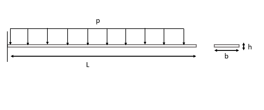
A cantilever beam is subjected to a distributed load, p. The beam is made of steel and modulus of elasticity and Poisson’s ratio of the material is known. Height, width and length of the beam is also given. We will calculate the deflection of the cantilever beam.

Properties and BC Value

Material Properties	Geometric Properties	Loading
E = 207 GPa	L = 0.2 m, b = 0.02 m, h = 0.002 m	p = 100 N/m
v = 0.3	I = \(0.01333\times10^{-9}\)

2.MODEL SETUP AND SOLUTION

The following sections describe the setup and solution steps for this tutorial:

2.1.Preparation

2.2.General Settings

2.3.Geometry/Mesh

2.4.Material

2.5.Boundary Conditions

2.6.Solution

2.7.Processing

2.8.Post-Processing

2.1. Preparation

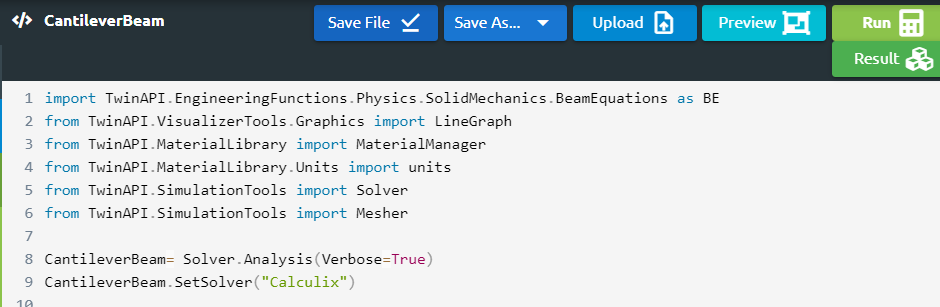
1.First we will import our libraries, that we will use almost in each tutorial, from Simularge Libraries to our empty Python page .

from TwinAPI.SimulationTools import Solver
from TwinAPI.SimulationTools import Mesher

Material properties are significant factors that affect the result. Therefore, we should be able to define them easily. Below I will explain how to use and write Material Library elaborately. Furthermore, the libraries which has to be imported for this problem is given below.

from TwinAPI.MaterialLibrary import MaterialManager
from TwinAPI.MaterialLibrary.Units import units

Now we will import Engineering Functions library. With this library we can calculate the theoritical result of our problem and then compare it with the result obtained from the analysis. We also import the necessary library for graphs because we want to represent and compare our results with a graph.

import TwinAPI.EngineeringFunctions.Physics.SolidMechanics.BeamEquations as BE
from TwinAPI.VisualizerTools.Graphics import LineGraph

2.2. General Settings

After the necessary libraries are imported into the analysis, the analysis is defined.

1.Define the name of the analysis as “CantileverBeam”

CantileverBeam= Solver.Analysis(Verbose=True)

2.Calculix is used for solid mechanics problems in TwinAPI. Hence, we define Calculix as the solver for this analysis.

CantileverBeam.SetSolver("Calculix")

Analysis is defined successfully into TwinAPI system.

2.3. Geometry/Mesh

There are two different options to define the geometry on TwinAPI system. You can create the geometry on TwinAPI by using Mesher Library which is one of Simularge libraries or you can import your own CAD geometry.

    L = 0.2
    b = 0.02
    h = 0.002
    NodeX = 401
    NodeY = 5
    NodeZ = 41
    directionX = ">"
    directionY = "<>"
    directionZ = "<>"
    TypeX = "uniform"
    TypeY = "uniform"
    TypeZ = "uniform"
    TransX = 0
    TransY = 0
    TransZ = 0

    box=Mesher.box(L,NodeX,TypeX,directionX,h,NodeY,TypeY,directionY, b,NodeZ,TypeZ,directionZ, TransX,TransY,TransZ)

With the script given above, you can create your geometry and mesh.

L= Length in the x-direction

NodeX= Node Number in the x-direction

directionX= Aspect

TypeX= Mesh type inthe x-direction.

TransX= Translation in the x-irection

All of given above is valid for y- and z-direction.

We create a box geometry with the name “box” from given inputs. Since the problem is solved in Abaqus using mesh size of 0.5 mm (problem reference is at the end of the page), number of nodes in our analysis is determined accordingly.

Note

We told you that you can also create this geometry by importing 3D CAD file apart from using MESHER. Code should be written like this;

Box1=Mesher.MeshFromCad('Box.step',20000,1,1e4,SurfaceExtract=True)

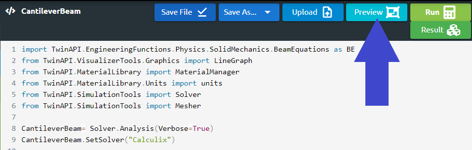
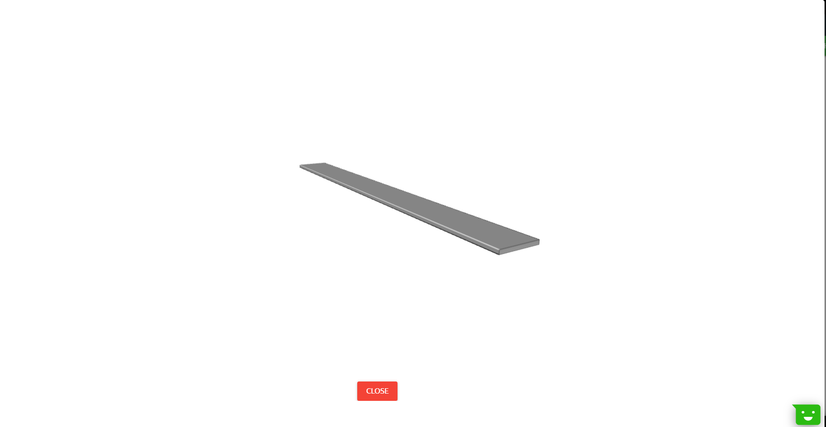
If we are not sure how the created geometry is and want to see the geometry before starting analysis;

Click Preview Button

2.4. Material

Before we start, there are lots of parameters which will affect the result of the problem. We are going to explain which parameters are required for this problem and some parameter instances will be given.

We call the Material class in the Material Manager library and name the material as “TwinAPI”. At the same time, we give the information that the material behaves as steel by typing “steel”.

Our material will behave elastically, therefore we type “Elastic”. Modulus of elasticity and Poisson’s ratio is required for this problem.

material = MaterialManager.Material("TwinAPI","steel")

material.SetMechanicType("Elastic")
material.SetMechanicData("youngsModulus",207e9,units["pa"])
material.SetMechanicData("poissonsRatio",0.3)

Other examples of parameters in Material Library are given below.

material.SetGeneralData("density", 7860, units["kg/m3"])

After defining the material into our system, we should combine geometry defined above and material using AddPart.

CantileverBeam.AddPart(box,material)

CantileverBeam.Assemble()

2.5. Boundary Conditions

After adding material and geometry to the analysis, we are ready to set the boundary conditions.

1.First of all, we will create a step with the name “Step1”.

Step1=Solver.CreateStep("new")

2.We need to choose whether this step is computed depending on time or not. Since our problem is steady-state, the code below should be used.

Step1.Time("SteadyState",[0,0.5,1])

If the problem was transient, type of the problem and time for the analysis would be written in a similar manner to the code given below.

Step1.Time("Transient",[0,10,0.1])

3.Since a cantilever beam has a fixed support at one end, we define the boundary conditions as given below. We define the load as “Pressure” and the distributed load is divided by the width of the beam to calculate the pressure.

Step1.AddBC("Fix",[box.right],[("X",0)],"")
Step1.AddBC("Fix",[box.right],[("Y",0)],"")
Step1.AddBC("Fix",[box.right],[("Z",0)],"")

Step1.AddBC("Pressure",[box.top],[("Y",-100/0.02)],"N/m2")

2.6. Solution

After defining our boundary conditions, we need to combine our defined domain and the steps containing boundary conditions.To complete this task;

CantileverBeam.Build([Step1])

Now,the problem is ready to be solved.

CantileverBeam.Solve()

After completing the analysis, we will calculate the theoritical solution using Engineering Functions library in TwinAPI.

distLoad = 100
elasticModulus = 207e9
inertia = 0.01333e-9

maxDeflection=BE.CDL(distLoad,elasticModulus,inertia,L,'max_deflection')
elasticCurve=BE.CDL(distLoad,elasticModulus,inertia,length,'elastic_curve')

Let’s review what we have done.

2.7. Processing

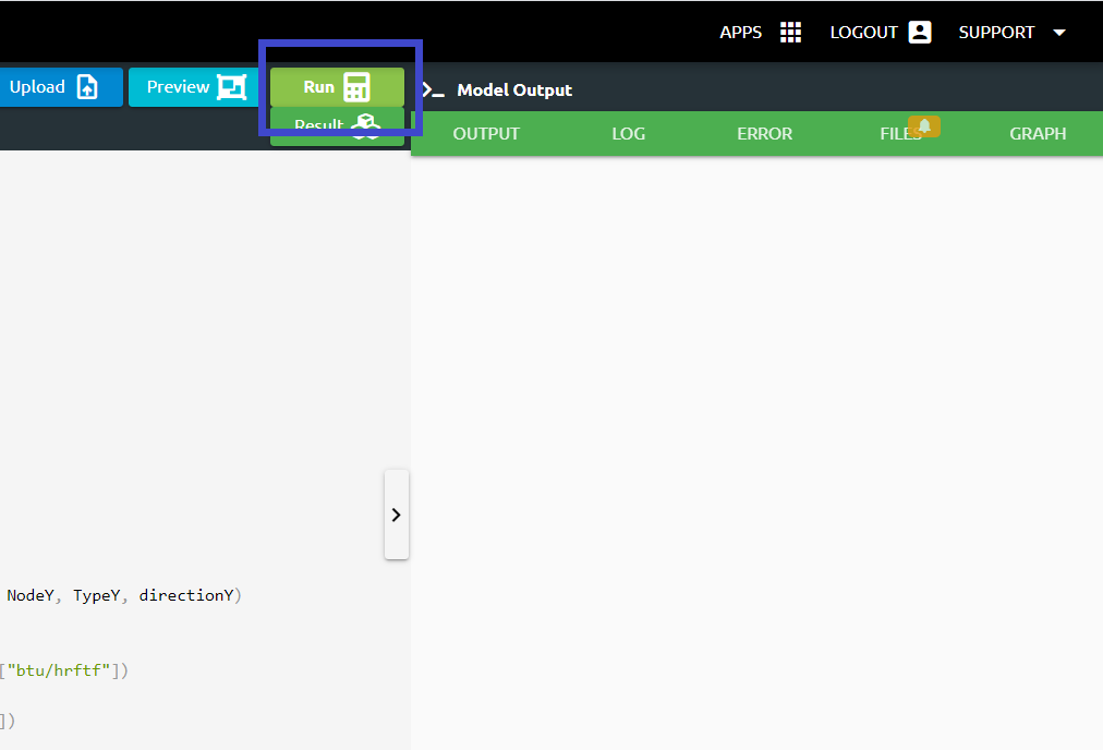
1. Click Run Button and gears will rotate on the right side while problem is being solved.

2.8. Post-Processing

2.After problem solved;

We can see the result;

Click Result Button

3.If we want to see the detailed result of the problem;

Output tab shows us the results that we desire to see.

disp=CantileverBeam.Result(Variable="Displacement Y", Loc=[0.2,0.001,0.1])
print("Theoritical Value of Max Deflection: {0:0.5f}".format(maxDeflection*1000), "mm")
print("Max Deflection:", disp[0]*1000, "mm")

Log tab tells us respectively what happened in the analysis.

Error tab shows us if there is an error in the script, it tells us what the error is and where it is.

Files tab includes the files imported using Upload button.

Graph tab shows us analysis result viewed graphically.

import numpy

Length=numpy.linspace(0,0.2,100)
Disp=[]
for xLoc in numpy.linspace(0,0.2,100):
    Disp.append(-1*(CantileverBeam.Result(Variable="Displacement Y", Loc=[xLoc,0.001,0.1])[0]))

fastMultiplePlot = LineGraph("Deflection of a Cantilever Beam")
fastMultiplePlot.Plot([{"Analysis": numpy.linspace(0,0.2,100)}, {"Theoritical Result": numpy.linspace(0,0.2,100)}],\
    [{"Analysis": Disp}, {"Target": v(numpy.linspace(0,0.2,100))}])

3.SUMMARY

In this tutorial, we learned how to set up and solve a problem involving a cantilever beam. We also learned how to perform postprocessing in an engineering manner.

The table given below shows comparison of theoritical result, the result obtained from Abaqus and the result obtained from TwinAPI.

Comparison

SOLID MODEL	Target	ABAQUS	SIMULARGE-TwinAPI	Ratio: SIMULARGE/Target	Ratio: SIMULARGE/ABAQUS
Maximum Deflection, mm	7.248 mm	7.63 mm	7.62 mm	1.05	1.00

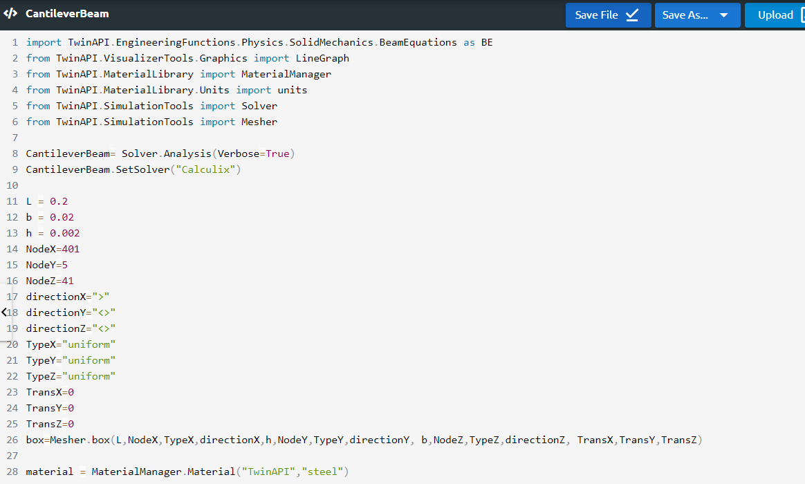
4. SOURCE CODE

import TwinAPI.EngineeringFunctions.Physics.SolidMechanics.BeamEquations as BE
from TwinAPI.VisualizerTools.Graphics import LineGraph
from TwinAPI.MaterialLibrary import MaterialManager
from TwinAPI.MaterialLibrary.Units import units
from TwinAPI.SimulationTools import Solver
from TwinAPI.SimulationTools import Mesher

CantileverBeam= Solver.Analysis(Verbose=True)
CantileverBeam.SetSolver("Calculix")

L = 0.2
b = 0.02
h = 0.002
NodeX=401
NodeY=5
NodeZ=41
directionX=">"
directionY="<>"
directionZ="<>"
TypeX="uniform"
TypeY="uniform"
TypeZ="uniform"
TransX=0
TransY=0
TransZ=0
box=Mesher.box(L,NodeX,TypeX,directionX,h,NodeY,TypeY,directionY, b,NodeZ,TypeZ,directionZ, TransX,TransY,TransZ)

material = MaterialManager.Material("TwinAPI","steel")

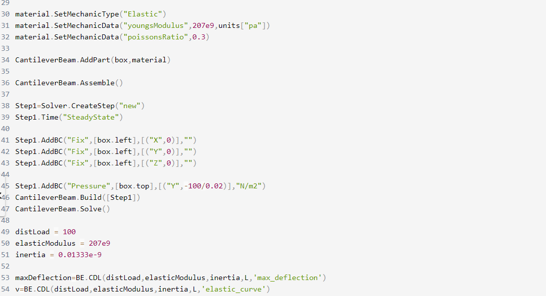
material.SetMechanicType("Elastic")
material.SetMechanicData("youngsModulus",207e9,units["pa"])
material.SetMechanicData("poissonsRatio",0.3)

CantileverBeam.AddPart(box,material)

CantileverBeam.Assemble()

Step1=Solver.CreateStep("new")
Step1.Time("SteadyState")

Step1.AddBC("Fix",[box.left],[("X",0)],"")
Step1.AddBC("Fix",[box.left],[("Y",0)],"")
Step1.AddBC("Fix",[box.left],[("Z",0)],"")

Step1.AddBC("Pressure",[box.top],[("Y",-100/0.02)],"N/m2")
CantileverBeam.Build([Step1])
CantileverBeam.Solve()

distLoad = 100
elasticModulus = 207e9
inertia = 0.01333e-9

maxDeflection=BE.CDL(distLoad,elasticModulus,inertia,L,'max_deflection')
v=BE.CDL(distLoad,elasticModulus,inertia,L,'elastic_curve')

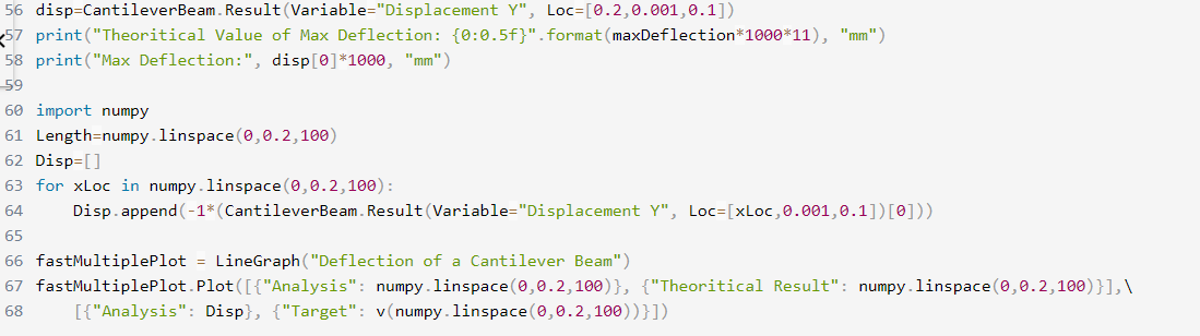
disp=CantileverBeam.Result(Variable="Displacement Y", Loc=[0.2,0.001,0.1])
print("Theoritical Value of Max Deflection: {0:0.5f}".format(maxDeflection*1000*11), "mm")
print("Max Deflection:", disp[0]*1000, "mm")

import numpy
Length=numpy.linspace(0,0.2,100)
Disp=[]
for xLoc in numpy.linspace(0,0.2,100):
    Disp.append(-1*(CantileverBeam.Result(Variable="Displacement Y", Loc=[xLoc,0.001,0.1])[0]))

fastMultiplePlot = LineGraph("Deflection of a Cantilever Beam")
fastMultiplePlot.Plot([{"Analysis": numpy.linspace(0,0.2,100)}, {"Theoritical Result": numpy.linspace(0,0.2,100)}],\
    [{"Analysis": Disp}, {"Target": v(numpy.linspace(0,0.2,100))}])

Keywords: Maximum Deflection, Cantilever Beam, Distributed Load

Problem Reference: http://www.7abaqus.com/analysis-of-cantilever-beam-under-pressure-loading-using-solid-shell-and-beam-elements-in-abaqus-software-abaqus-vs-exact-solution/

Author: Ilknur Akica